Continuity equation derivation in fluid mechanics with applications

General Concept of Fluid Flow

One way of describing the motion of a fluid is to divide the fluid into infinitesimal volume elements, which we may call fluid particles, and to follow the motion of each particle. If we knew the forces acting on each fluid particle, we could then solve for the coordinates and velocities of each particle as functions of the time. This procedure, which is a direct generalization of particle mechanics, was first developed by Joseph Louis Lagrange (1736 – 1813). Because the number of fluid particles is generally very large, using this method is a formidable task.

There is a different treatment, developed by Leonhard Euler (1707 – 1783), that is more convenient for most purposes. In it we give up the attempt to specify the history of each fluid particle and instead specify the density and the velocity of the fluid at each point in space at each instant of time. This is the method we shall use. We describe the motion of the fluid by specifying the density ρ(x,y,z,t) and the velocity v( x,y,z,t) at the point x,y,z at the time t. We thus focus our attention on what is happening at a particular point in space at a particular time, rather than on what is happening to a particular fluid particle. Any quantity used in describing the state of the fluid, for example, the pressure p, will have a definite value at each point in space and at each instant of time. Although this description of fluid motion focuses attention on a point in space rather than on a fluid particle, we cannot avoid following the fluid particles themselves, at least for short time intervals dt. After all, the laws of mechanics apply to particles and not to points in space.

We first consider some general characteristics of fluid flow.

• Fluid flow can be steady or non-steady. We describe the flow in terms of the values of such variables at pressure, density, and flow velocity at every point of the fluid. If these variables are constant in time, the flow is said to be steady. The values of these variables will generally change from one point to another, but they do not change with time at any particular point. The condition can often be achieved at low flow speeds; a gently flowing stream is an example. In non-steady flow, as in a tidal bore, the velocities v are functions of the time. In the case of turbulent flow, such as rapids waterfall, the velocities vary erratically from point to point as well as from time to time.
• Fluid flow can be compressible or in-compressible. If the density ρ of a fluid is a constant, independent of x,y,z, and t, its flow is called in-compressible flow. Liquids can usually be considered as following in-compressible. But even for a highly compressible gas, the variation in density may be insignificant, and for practical purposes, we can consider its flow to be in-compressible. For example, in flights at speeds much lower than the speed of sound in air (described by subsonic aerodynamics), the flow of the air over the wings is nearly incompressible.

•  Viscosity in fluid motion is the analog of friction in the motion of solids. When a fluid flows such that no energy is dissipated through viscous forces, the flow is said to be non-viscous. In many cases, such as in lubrication problems, viscosity is extremely important; motor oils, for example, are rated according to their viscosity and their vibration with temperature. In other cases, the viscosity may be relatively unimportant, and by neglecting it we can use a simple description in terms of non-viscous flow.
•  If an element of the moving fluid does not rotate about an exit through the center of mass of the element, the flow is said to be irrotational. We can imagine a small paddle wheel immersed in the moving fluid. If the wheel moves without rotating, the motion is irrotational; otherwise, it is rotational. Note that a particular element of fluid can move in a circular path and still experience irrotational flow; an analogy is the motion of the hanging cars in a Ferris wheel – even though the wheel rotates; the people in the cars do not rotate about their center of mass. The vortex formed when water flows around a bathtub drain is an example of this kind of irrotational flow.
• The ideal fluid moves without turbulence. This implies that each element of the fluid has zero angular velocity about its center.

To simplify the mathematical description of fluid motion, we confine our discussion of fluid dynamics for the most part to the steady, in-compressible,non-viscous, irrotational flow. We run the danger, however, of making so many simplifying assumptions that we are no longer talking about a real fluid. Furthermore, it is sometimes difficult to decide whether a given property of a fluid- its viscosity, say – can be neglected in a particular situation. In spite of all this, the restricted analysis that we are going to give has wide application in practice, as we shall see.

What is Continuity equation in fluid mechanics?

“The product of the cross-sectional area of the pipe and the fluid speed at any point along the pipe is constant. This product is equal to the volume flow per second or simply flow rate.”

Mathematically it is represented as:

Continuity equation formula

Av = Constant

Continuity equation derivation

Consider a fluid flowing through a pipe of non-uniform size. The particles in the fluid move along the same lines in a steady flow.

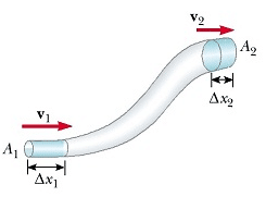
If we consider the flow for a short interval of time Δt, the fluid at the lower end of the pipe covers a distance Δx₁ with a velocity v₁, then:

Distance covered by the fluid = Δx₁ = v₁Δt

Let A₁ be the area of the cross-section of the lower end then the volume of the fluid that flows into the pipe at the lower end =V= A₁ Δx₁ = A₁ v₁  Δt

If ρ is the density of the fluid, then the mass of the fluid contained in the shaded region of the lower end of the pipe is:

Δm₁=Density × volume

Δm₁ = ρ₁A₁v₁Δt ——–(1)

Now the mass flux defined as the mass of the fluid per unit of time passing through any cross-section at the lower end is:

Δm_{1/Δt =}ρ₁A₁v₁

Mass flux at lower end = ρ₁A₁v_{1 ———————(2)}

If the fluid moves with velocity v₂ through the upper end of the pipe having cross-sectional area A₂ in time Δt, then the mass flux at the upper end is given by:

Δm_2/Δt = ρ₂A₂v₂ 

Mass flux at upper end =ρ₂A₂v_{2  ———————–(3)}

Since the flow is steady, so the density of the fluid between the lower and upper ends of the pipe does not change with time. Thus the mass flux at the lower end must be equal to the mass flux at the upper end so:

ρ₁A₁v_{1 =} ρ₂A₂v_{2  ———————-(4)}

In a more general form we can write :

ρ A v =constant

This relation describes the law of conservation of mass in fluid dynamics. If the fluid is incompressible, then density is constant for a steady flow of incompressible fluid so

 ρ₁ =ρ₂

Now equation (4) can be written as:

A₁ v_{1 =} A₂ v₂

In general:

A v = constant

If R is the volume flow rate then :

R = A v = constant

Watch also:

Read also:
Bernoulli’s equation
Viscosity
Terminal velocity